Direct

Introduction

This method attempts a direct integration of the Abel transform integral. It makes no assumptions about the data (apart from cylindrical symmetry), but it typically requires fine sampling to converge. Unlike other methods implemented in PyAbel, it can work with the data sampled on a non-uniform grid. Such methods are typically inefficient, but thanks to this Cython implementation (by Roman Yurchak), this “direct” method is competitive with the other methods.

How it works

The 1D forward and inverse Abel transforms

\[F(y) = 2 \int_y^\infty \frac{f(r)\,r\,dr}{\sqrt{r^2 - y^2}}, \quad f(r) = -\frac1\pi \int_r^\infty \frac{dF(y)}{dy} \frac{dy}{\sqrt{y^2 - r^2}}\]

can be expressed in the unified form

\[\begin{split}G(x) = \int_x^\infty \frac{g(r)\,dr}{\sqrt{r^2 - x^2}}, \quad g(r) = \begin{cases} 2rf(r) & \text{forward transform}, \\[0.5ex] -\dfrac1\pi \dfrac{F(r)}{dr} & \text{inverse transform}. \end{cases}\end{split}\]

The “direct” method prepares the corresponding \(g(r)\) from the input data. In case of the inverse transform, the derivative is taken numerically using numpy.gradient() or any user-defined numerical differentiation function.

The integration is then performed numerically using the trapezoidal rule (by default) or any user-defined numerical integration function. The numerical integration had to exclude the segment at the lower limit, where \(r = x\), and thus the integrand becomes infinite. This causes a systematic underestimation of the integral. To correct for this underestimation, the truncated numerical integral is by default supplemented with an analytical integral over the excluded segment, assuming that \(g(r)\) is locally linear:

\[g(r_i + dr) = g(r_i) + g'(r_i)\,dr, \quad g'(r_i) = \frac{g(r_{i+1}) - g(r_i)}{r_{i+1} - r_i},\]

so that

\[\begin{split}\begin{aligned} \int_{x_i}^{x_{i+1}} \frac{g(r)\,dr}{\sqrt{r^2 - x_i^2}} &= \operatorname{arccosh}\frac{x_{i+1}}{x_i} \cdot g(x_i) + \left(y - x_i \operatorname{arccosh}\frac{x_{i+1}}{x_i}\right) g'(x_i) = \\ &= \frac{[g(x_i) x_{i+1} + g(x_{i+1}) x_i] \ln\frac{x_{i+1} + y}{x_i} + [g(x_{i+1}) - g(x_i)] y} {x_{i+1} - x_i}, \end{aligned}\end{split}\]

where \(y = \sqrt{r^2 - x_i^2}\) with \(r = x_{i+1}\). The axial pixel has \(x_0 = 0\), so the above expressions also have singularities, but their analytical limit is simply

\[\int_0^{x_1} \frac{g(r)\,dr}{\sqrt{r^2 - 0^2}} = g'(0) x_1 = g(x_1),\]

necessarily assuming that \(g(0) = 0\), which is true for well-behaved functions \(f\) and \(F\) in the forward and inverse Abel transforms.

When to use it

When a robust forward transform is required, this method works quite well. It is not typically recommended for the inverse transform, but it can work well for smooth functions that are finely sampled. The sampling does not need to be uniform, so more points can be allocated to more important areas. Note, however, that abel.Transform and image-processing tools in PyAbel work only with uniform sampling, thus if you need to use them, it is recommended to resample the original data on a sufficiently fine uniform grid and use one of the more efficient transform methods.

How to use it

To complete the forward or inverse transform of a full image with the direct method, simply use the abel.Transform class:

abel.Transform(myImage, method='direct', direction='forward').transform
abel.Transform(myImage, method='direct', direction='inverse').transform

If you would like to access the Direct algorithm directly (to transform a right-side half-image, possibly with non-uniform sampling), you can use abel.direct.direct_transform().

Examples

Incomplete data

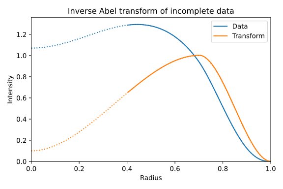
The transform integral for any \(x\) depends only on the function at \(r \geqslant x\), thus it is possible to transform incomplete data, with the signal near the symmetry axis unavailable or contaminated. (See also Example: rBasex beam block.)

Source code ▾

import matplotlib.pyplot as plt
from abel.direct import direct_transform
from abel.tools.analytical import TransformPair

ref = TransformPair(n=100, profile=4)

# take the data for r > r_min only
r_min = 0.4
n_min = int(ref.n * r_min)
cut_r = ref.r[n_min:]
cut_abel = ref.abel[n_min:]

# inverse Abel transform for r > r_min
cut_res = direct_transform(cut_abel, r=cut_r, direction='inverse')

plt.figure(figsize=(6, 4))
plt.title('Inverse Abel transform of incomplete data')
plt.xlabel('Radius')
plt.ylabel('Intensity')
plt.plot(ref.r, ref.abel, 'C0:')
plt.plot(cut_r, cut_abel, 'C0', label='Data')
plt.plot(ref.r, ref.func, 'C1:')
plt.plot(cut_r, cut_res, 'C1', label='Transform')
plt.xlim(0, 1)
plt.ylim(0, None)
plt.legend()
plt.tight_layout()
plt.show()

Non-uniform sampling

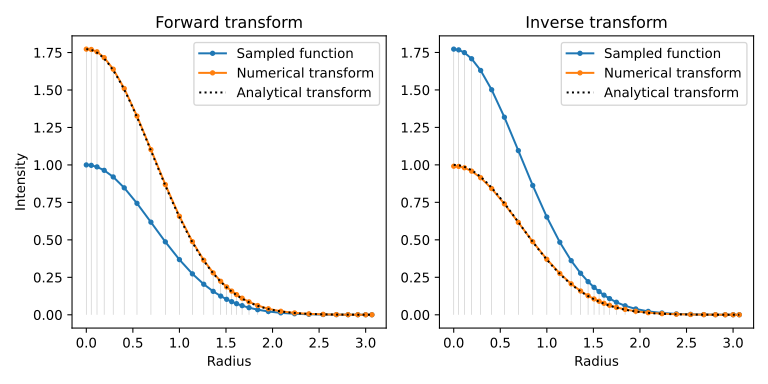
Forward and inverse Abel transforms of a Gaussian function, using denser sampling in the regions where the function curvature is larger. Only 30 samples are used here to make individual points discernible, but using more points will make the transform more accurate.

Source code ▾

import numpy as np
import matplotlib.pyplot as plt
from abel.tools.analytical import GaussianAnalytical
from abel.direct import direct_transform

# a Gaussian sampled on a non-uniform grid (denser in more curved regions)
n = 30
r = np.linspace(0, 3, n)
r -= 0.5 * np.sin(r * 4) / 4
f = np.exp(-r**2)

ref = GaussianAnalytical(100, r[-1], symmetric=False)

plt.figure(figsize=(8, 4))

plt.subplot(121)
plt.title('Forward transform')
fabel = direct_transform(f, r=r, direction='forward')
plt.xlabel('Radius')
plt.ylabel('Intensity')
plt.vlines(r, 0, fabel, lw=0.5, colors='0.8')
plt.plot(r, f, 'C0.-', label='Sampled function')
plt.plot(r, fabel, 'C1.-', label='Numerical transform')
plt.plot(ref.r, ref.abel, 'k:', label='Analytical transform')
plt.legend()

plt.subplot(122)
plt.title('Inverse transform')
f *= ref.abel[0]
iabel = direct_transform(f, r=r, direction='inverse')
plt.xlabel('Radius')
plt.vlines(r, 0, f, lw=0.5, colors='0.8')
plt.plot(r, f, 'C0.-', label='Sampled function')
plt.plot(r, iabel, 'C1.-', label='Numerical transform')
plt.plot(ref.r, ref.func, 'k:', label='Analytical transform')
plt.legend()

plt.tight_layout()
plt.show()

Custom differentiation and integration

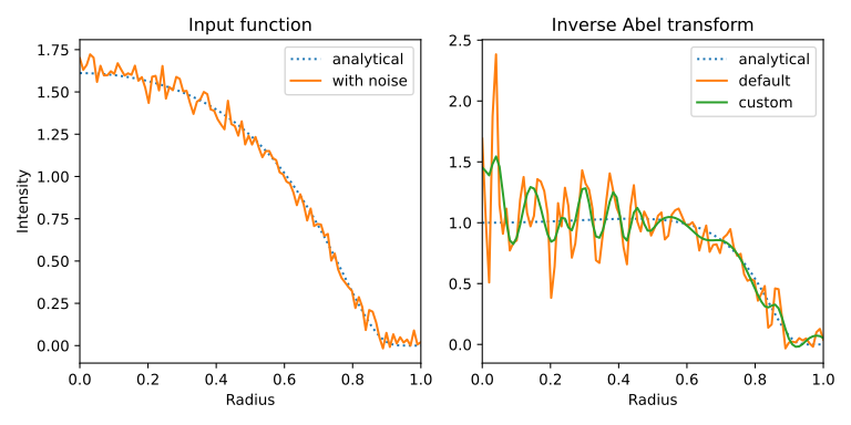
As mentioned above, the default numerical differentiation and integration methods can be replaced by user-defined Python functions. This example estimates the derivative from a smoothing spline fit to the noisy data and uses the composite Simpson’s rule for numerical integration.

Source code ▾

import numpy as np
import scipy
import matplotlib.pyplot as plt
from abel.tools.analytical import TransformPair
from abel.direct import direct_transform

ref = TransformPair(100, profile=6)
noise = 0.05  # RMS intensity of additive noise
tol = 0.04    # RMS tolerance for derivative smoothing

noisy_abel = np.random.RandomState(0).normal(ref.abel, noise)

plt.figure(figsize=(8, 4))

plt.subplot(121)
plt.title('Input function')
plt.xlabel('Radius')
plt.ylabel('Intensity')
plt.plot(ref.r, ref.abel, ':', label='analytical')
plt.plot(ref.r, noisy_abel, label='with noise')
plt.xlim(0, 1)
plt.legend()

# inverse transform using default differentiation and integration
default = direct_transform(noisy_abel, r=ref.r, direction='inverse')

# example of a custom derivative function
def derivative(f, x):
    out = np.empty_like(f)
    for row in range(f.shape[0]):
        # create a smoothing spline
        smoothed = scipy.interpolate.make_splrep(x, f[row], s=tol**2 * f.size)
        # sample its first derivative on the original grid
        out[row] = smoothed(x, 1)
    return out

# example of a custom integral function
def integral(f, x):
    return scipy.integrate.simpson(f, x, axis=1)

# inverse transform using custom derivative and integral
custom = direct_transform(noisy_abel, r=ref.r, direction='inverse',
                          derivative=derivative, integral=integral,
                          backend='Python')

plt.subplot(122)
plt.title('Inverse Abel transform')
plt.xlabel('Radius')
plt.plot(ref.r, ref.func, ':', label='analytical')
plt.plot(ref.r, default, label='default')
plt.plot(ref.r, custom, label='custom')
plt.xlim(0, 1)
plt.legend()

plt.tight_layout()
plt.show()

Tip

The derivative function is called only once for the input image, but the integral function is called for each column of the transformed image and thus should be implemented efficiently, as otherwise the whole transform might become very slow.