Example: Anisotropy parameter

# -*- coding: utf-8 -*-
from __future__ import division
from __future__ import print_function
from __future__ import unicode_literals

import numpy as np
import abel
import bz2

import matplotlib.pylab as plt

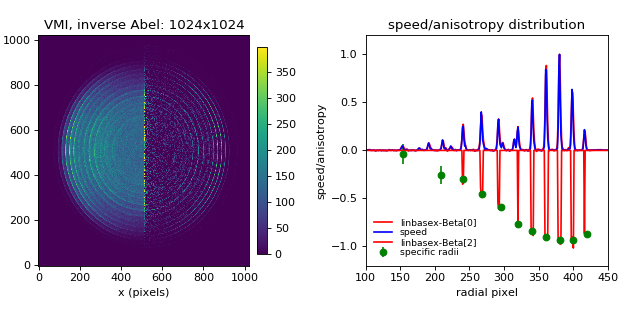
# Demonstration of two techniques to determine the anisotropy parameter
# (a) directly, using `linbasex`
# (b) from the inverse Abel transformed image

# Load image as a numpy array
imagefile = bz2.BZ2File('data/O2-ANU1024.txt.bz2')
IM = np.loadtxt(imagefile)
# use scipy.misc.imread(filename) to load image formats (.png, .jpg, etc)

# === linbasex transform ===================================
legendre_orders = [0, 2, 4]  # Legendre polynomial orders
proj_angles = range(0, 180, 10)  # projection angles in 10 degree steps
radial_step = 1  # pixel grid
smoothing = 0.9  # smoothing 1/e-width for Gaussian convolution smoothing
threshold = 0.2  # threshold for normalization of higher order Newton spheres
clip = 0  # clip first vectors (smallest Newton spheres) to avoid singularities

# linbasex method - center and center_options ensure image has odd square shape
LIM = abel.Transform(IM, method='linbasex', center='slice',
                     center_options=dict(square=True),
                     transform_options=dict(basis_dir=None,
                     proj_angles=proj_angles, radial_step=radial_step,
                     smoothing=smoothing, threshold=threshold, clip=clip,
                     return_Beta=True, verbose=True))


# === Hansen & Law inverse Abel transform ==================
HIM = abel.Transform(IM, center="slice", method="hansenlaw",
                     symmetry_axis=None, angular_integration=True)

# speed distribution
radial, speed = HIM.angular_integration

# normalize to max intensity peak
speed /= speed[200:].max()  # exclude transform noise near centerline of image

# PAD - photoelectron angular distribution from image ======================
# Note: `linbasex` provides the anisotropy parameter directly LIM.Beta[1]
#       here we extract I vs theta for given radial ranges
#       and use fitting to determine the anisotropy parameter
#
# radial ranges (of spectral features) to follow intensity vs angle
# view the speed distribution to determine radial ranges
r_range = [(145, 162), (200, 218), (230, 250), (255, 280), (280, 310),
           (310, 330), (330, 350), (350, 370), (370, 390), (390, 410),
           (410, 430)]

# anisotropy parameter from image for each tuple r_range
Beta, Amp, Rmid, Ivstheta, theta =\
              abel.tools.vmi.radial_integration(HIM.transform, r_range)

# OR  anisotropy parameter for ranges (0, 20), (20, 40) ...
# Beta_whole_grid, Amp_whole_grid, Radial_midpoints =\
#                         abel.tools.vmi.anisotropy(AIM.transform, 20)

# plots of the analysis
fig = plt.figure(figsize=(8, 4))
ax1 = plt.subplot(121)
ax2 = plt.subplot(122)

# join 1/2 raw data : 1/2 inversion image
rows, cols = IM.shape
c2 = cols//2
vmax = IM[:, :c2-100].max()
AIM = HIM.transform
AIM *= vmax/AIM[:, c2+100:].max()
JIM = np.concatenate((IM[:, :c2], AIM[:, c2:]), axis=1)

# Plot the image data VMI | inverse Abel
im1 = ax1.imshow(JIM, origin='lower', aspect='auto', vmin=0, vmax=vmax)
fig.colorbar(im1, ax=ax1, fraction=.1, shrink=0.9, pad=0.03)
ax1.set_xlabel('x (pixels)')
ax1.set_ylabel('y (pixels)')
ax1.set_title('VMI, inverse Abel: {:d}x{:d}'.format(rows, cols))

# Plot the 1D speed distribution
ax2.plot(LIM.Beta[0], 'r-', label='linbasex-Beta[0]')
ax2.plot(speed, 'b-', label='speed')
# Plot anisotropy parameter, attribute Beta[1], x speed
ax2.plot(LIM.Beta[1], 'r-', label='linbasex-Beta[2]')
BetaT = np.transpose(Beta)
ax2.errorbar(Rmid, BetaT[0], BetaT[1], fmt='o', color='g',
             label='specific radii')
# ax2.plot(Radial_midpoints, Beta_whole_grid[0], '-g', label='stepped')
ax2.axis(xmin=100, xmax=450, ymin=-1.2, ymax=1.2)
ax2.set_xlabel('radial pixel')
ax2.set_ylabel('speed/anisotropy')
ax2.set_title('speed/anisotropy distribution')
ax2.legend(frameon=False, labelspacing=0.1, numpoints=1, loc=3,
           fontsize='small')

plt.subplots_adjust(left=0.06, bottom=0.17, right=0.95, top=0.89,
                    wspace=0.35, hspace=0.37)

# Save a image of the plot
plt.savefig("plot_example_PAD.png", dpi=100)

# Show the plots
plt.show()

(Source code, png, hires.png, pdf)