Example: All_Dribinski

# -*- coding: utf-8 -*-

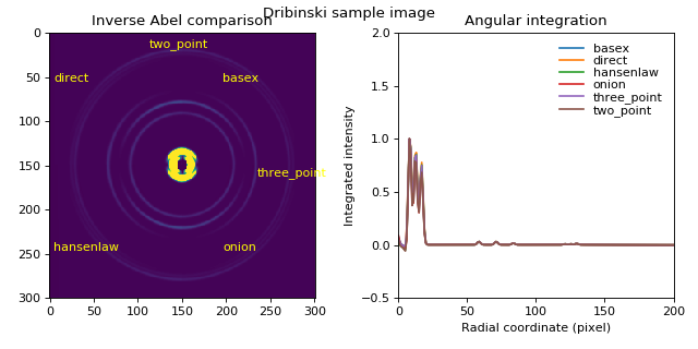
# This example compares the available inverse Abel transform methods
# for the Ominus sample image
#
# Note it transforms only the Q0 (top-right) quadrant
# using the fundamental transform code

from __future__ import absolute_import
from __future__ import division
from __future__ import print_function
from __future__ import unicode_literals

import numpy as np
import abel

import collections
import matplotlib.pylab as plt
from time import time

fig, (ax1,ax2) = plt.subplots(1, 2, figsize=(8,4))

# inverse Abel transform methods -----------------------------
#   dictionary of method: function()

transforms = {
  "direct": abel.direct.direct_transform,
  "hansenlaw": abel.hansenlaw.hansenlaw_transform,
  "onion": abel.dasch.onion_peeling_transform,
  "basex": abel.basex.basex_transform,
  "three_point": abel.dasch.three_point_transform,
  "two_point": abel.dasch.two_point_transform,
}

# sort dictionary:
transforms = collections.OrderedDict(sorted(transforms.items()))
# number of transforms:
ntrans = np.size(transforms.keys())

IM = abel.tools.analytical.SampleImage(n=301, name="dribinski").image

h, w = IM.shape

# forward transform:
fIM = abel.Transform(IM, direction="forward", method="hansenlaw").transform

Q0, Q1, Q2, Q3 = abel.tools.symmetry.get_image_quadrants(fIM, reorient=True)

Q0fresh = Q0.copy()    # keep clean copy
print ("quadrant shape {}".format(Q0.shape))

# process Q0 quadrant using each method --------------------

iabelQ = []  # keep inverse Abel transformed image

for q, method in enumerate(transforms.keys()):

    Q0 = Q0fresh.copy()   # top-right quadrant of O2- image

    print ("\n------- {:s} inverse ...".format(method))
    t0 = time()

    # inverse Abel transform using 'method'
    IAQ0 = transforms[method](Q0, direction="inverse", basis_dir='bases')

    print ("                    {:.4f} sec".format(time()-t0))

    iabelQ.append(IAQ0)  # store for plot

    # polar projection and speed profile
    radial, speed = abel.tools.vmi.angular_integration(IAQ0, origin=(0, 0), Jacobian=False)

    # normalize image intensity and speed distribution
    IAQ0 /= IAQ0.max()
    speed /= speed.max()

    # method label for each quadrant
    annot_angle = -(45+q*90)*np.pi/180  # -ve because numpy coords from top
    if q > 3:
        annot_angle += 50*np.pi/180    # shared quadrant - move the label
    annot_coord = (h/2+(h*0.9)*np.cos(annot_angle)/2 -50,
                   w/2+(w*0.9)*np.sin(annot_angle)/2)
    ax1.annotate(method, annot_coord, color="yellow")

    # plot speed distribution
    ax2.plot(radial, speed, label=method)

# reassemble image, each quadrant a different method

# for < 4 images pad using a blank quadrant
blank = np.zeros(IAQ0.shape)
for q in range(ntrans, 4):
    iabelQ.append(blank)

# more than 4, split quadrant
if ntrans == 5:
    # split last quadrant into 2 = upper and lower triangles
    tmp_img = np.tril(np.flipud(iabelQ[-2])) +\
              np.triu(np.flipud(iabelQ[-1]))
    iabelQ[3] = np.flipud(tmp_img)

im = abel.tools.symmetry.put_image_quadrants((iabelQ[0], iabelQ[1],
                                              iabelQ[2], iabelQ[3]),
                                              original_image_shape=IM.shape)

ax1.imshow(im, vmin=0, vmax=0.15)
ax1.set_title('Inverse Abel comparison')


ax2.set_xlim(0, 200)
ax2.set_ylim(-0.5,2)
ax2.legend(loc=0, labelspacing=0.1, frameon=False)
ax2.set_title('Angular integration')
ax2.set_xlabel('Radial coordinate (pixel)')
ax2.set_ylabel('Integrated intensity')


plt.suptitle('Dribinski sample image')

plt.tight_layout()
plt.savefig('plot_example_all_dribinski.png', dpi=100)
plt.show()

(Source code, png, hires.png, pdf)