Circularization of Images
Background
While the Abel transform only assumes cylindrical symmetry, often the objects to be transformed also have some degree of spherical symmetry, (i.e., features that appear at a constant radius for all angles) and thus the 2D projection should be perfectly circular. Experimental images may have distortions in the circular charged particle energy structure, due to, for example, stray magnetic fields, or optical distortion of the camera lens that images the particle detector. The effect of distortion is to degrade the radial (or velocity or kinetic energy) resolution, since a particular energy peak will “walk” in radial position, depending on the particular angular position on the detector. Imposing a physical circular distribution of particles, may substantially improve the kinetic energy resolution, at the expense of uncertainly in the absolution kinetic-energy position of the transition.
Approach
The algorithm is implemented in abel.tools.circularize.circularize_image()
compares the radial positions of strong features in angular slice intensity profiles. i.e. follow the radial position of a peak as a function of angle. A linear correction is applied to the radial grid to align the peak at each angle.
 before     after
   ^         ^    slice0
     ^       ^    slice1
   ^         ^    slice2
  ^          ^    slice3
   :         :
    ^        ^    slice#
radial peak position
Peak alignment is achieved through a radial scaling factor \(R_i(actual) = R_i \times scalefactor_i\). The scalefactor is determined by a choice of methods, argmax, where \(scalefactor_i = R_0/R_i\), with \(R_0\) a reference peak. Or lsq, which directly determines the radial scaling factor that best aligns adjacent slice intensity profiles.
This is a simplified radial scaling version of the algorithm described in J. R. Gascooke and S. T. Gibson and W. D. Lawrance: ‘A “circularisation” method to repair deformations and determine the centre of velocity map images’ J. Chem. Phys. 147, 013924 (2017).
Implementation
Cartesian \((y, x)\) image is converted to a polar coordinate image \((r, \theta)\) for easy slicing into angular blocks. Each radial intensity profile is compared with its adjacent slice, providing a radial scaling factor that best aligns the two intensity profiles.
The set of radial scaling factors, for each angular slice, is then spline interpolated to correct the \((y, x)\) grid, and the image remapped to an unperturbed grid.
How to use it
The circularize_image() function is called directly
IMcirc, angle, radial_correction, radial_correction_function =\
    abel.tools.circularize.circularize_image(IM, method='lsq',\
    center='slice', dr=0.5, dt=0.1, return_correction=True)
The main input parameters are the image IM, and the number of angular slices, to use, which is set by \(2\pi/dt\). The default dt = 0.1 uses ~63 slices. This parameter determines the angular resolution of the distortion correction function, but is limited by the signal to noise loss with smaller dt. Other parameters may help better define the radial correction function.
Warning
Ensure the returned radial_correction vs angle data is a well behaved function.
See the example, below, bottom left figure. If necessary limit the radial_range=(Rmin, Rmax), or change the value of the spline smoothing parameter.
Example
import numpy as np
import matplotlib.pyplot as plt
import abel
import scipy.interpolate
#######################################################################
#
# example_circularize_image.py
#
# O- sample image -> forward Abel + distortion = measured VMI
# measured VMI -> inverse Abel transform -> speed distribution
# Compare disorted and circularized speed profiles
#
#######################################################################
# sample image -----------
IM = abel.tools.analytical.SampleImage(n=511, name='Ominus', sigma=2).image
# forward transform == what is measured
IMf = abel.Transform(IM, method='hansenlaw', direction="forward").transform
# flower image distortion
def flower_scaling(theta, freq=2, amp=0.1):
return 1 + amp*np.sin(freq*theta)**4
# distort the image
IMdist = abel.tools.circularize.circularize(IMf,
radial_correction_function=flower_scaling)
# circularize ------------
IMcirc, sla, sc, scspl = abel.tools.circularize.circularize_image(IMdist,
method='lsq', dr=0.5, dt=0.1, smooth=0, return_correction=True)
# inverse Abel transform for distored and circularized images ---------
AIMdist = abel.Transform(IMdist, method="three_point",
transform_options=dict(basis_dir='bases')).transform
AIMcirc = abel.Transform(IMcirc, method="three_point",
transform_options=dict(basis_dir='bases')).transform
# respective speed distributions
rdist, speeddist = abel.tools.vmi.angular_integration(AIMdist, dr=0.5)
rcirc, speedcirc = abel.tools.vmi.angular_integration(AIMcirc, dr=0.5)
# note the small image size is responsible for the slight over correction
# of the background near peaks
row, col = IMcirc.shape
# plot --------------------
fig, axs = plt.subplots(2, 2, figsize=(8, 8))
fig.subplots_adjust(wspace=0.5, hspace=0.5)
extent = (np.min(-col//2), np.max(col//2), np.min(-row//2), np.max(row//2))
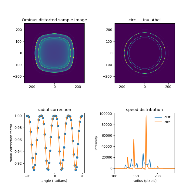
axs[0, 0].imshow(IMdist, aspect='auto', origin='lower', extent=extent)
axs[0, 0].set_title("Ominus distorted sample image")
axs[0, 1].imshow(AIMcirc, vmin=0, aspect='auto', origin='lower',
extent=extent)
axs[0, 1].set_title("circ. + inv. Abel")
axs[1, 0].plot(sla, sc, 'o')
ang = np.arange(-np.pi, np.pi, 0.1)
axs[1, 0].plot(ang, scspl(ang))
axs[1, 0].set_xticks([-np.pi, 0, np.pi])
axs[1, 0].set_xticklabels([r"$-\pi$", "0", r"$\pi$"])
axs[1, 0].set_xlabel("angle (radians)")
axs[1, 0].set_ylabel("radial correction factor")
axs[1, 0].set_title("radial correction")
axs[1, 1].plot(rdist, speeddist, label='dist.')
axs[1, 1].plot(rcirc, speedcirc, label='circ.')
axs[1, 1].axis(xmin=100, xmax=240)
axs[1, 1].set_title("speed distribution")
axs[1, 1].legend(frameon=False)
axs[1, 1].set_xlabel('radius (pixels)')
axs[1, 1].set_ylabel('intensity')
plt.savefig("plot_example_circularize_image.png", dpi=75)
plt.show()
(Source code, png, hires.png, pdf)